Sebastian Pokutta's Blog

On the polyhedral inapproximability of the SDP cone

I was at HPOPT in Delft last week which was absolutely great and I would like to thank Mirijam Dür and Frank Vallentin for the organization and providing us with such an inspirational atmosphere. I talked On the complexity of polytopes and extended formulations which was based on two recent papers (see [1] and [2] below) which are joint work with Gábor Braun, Samuel Fiorini, Serge Massar, David Steurer, Hans Raj Tiwary and Ronald de Wolf. One of the question that came up repeatedly was the statement for the inapproximability of the SDP cone via Linear Programming and its consequences. This is what this brief post will be about; I simplify and purposefully imprecise a few things for the sake of exposition.

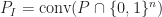
For a closed convex body $K$ containing $0$ there is a natural notion of appoximating $K$ within a factor of $(1+ \epsilon)$ with $\epsilon > 0$ . We can simplify define $(1+\epsilon) K = \{ (1+\epsilon) x \mid x \in K\}$ . This notion is compatible with the notion of approximating the maximum value of a (say, nonnegative) linear objective from the outside over $K$ within a factor of $1+\epsilon$ . For this observe that

$\frac{\max_{x \in (1+\epsilon) K} cx}{\max_{x \in K} cx} = \frac{\max_{x \in K} (1+\epsilon) cx}{\max_{x \in K} cx} \leq (1+\epsilon)$

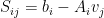
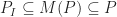
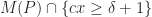
What one can show now is that there exists a pair polyhedra $P \subseteq Q$ where $P = COR(n) = conv\{bb^T \mid b \in \{0,1\}^n\}$ is the correlation polytope (also called boolean quadric polytope) and $Q$ is given by the valid inequalities $<2 diag(a) - aa^T,x> \leq 1$ for all $a \in \{0,1\}^n$ . This pair of polyhedra has the property that for any other polyhedron $T$ so that $P \subseteq T \subseteq (1+\epsilon) Q$ it follows that one needs a super-polynomial number of inequalities in any extended formulation of $T$ and $\epsilon$ can be here as large as $O(n^\beta)$ with $\beta < 1/2$ . This follows from a modification of Razborov’s well-known rectangle corruption lemma.

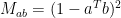
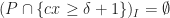
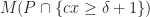
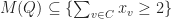
On the other hand, there exists a spectrahedron $S \in \mathbb R^{n \times n}$ sandwiched between $P$ and $Q$ , i.e., $P \subseteq S \subseteq Q$ where $S$ is the projection of an affine space intersected with the cone of $n+1 \times n+1$ psd matrices. In particular $P \subseteq S \subseteq (1+\epsilon)S \subseteq (1+\epsilon)Q$ . Now, if $K$ is a polyhedron so that $S \subseteq K \subseteq (1+\epsilon) S$ it follows that $K$ needs a super polynomial number of inequalities in any extended formulation for any $\epsilon = O(n^\beta)$ with $\beta < 1/2$ . In consequence, there exists a spectrahedron $S$ with small SDP extension complexity that cannot be well approximated by any polyhedron. If now the SDP cone could be approximated well (in sense similar to the one for the SOCP cone, see [3]), so could this particular spectrahedron. This is inapproximability is in contrast to the case of SOCP cone which can be approximated arbitrarily well with a polynomial number of inequalities (see [3] for a precise statement). (Note that we can add the nonnegativity constraints to obtain the same statements for polytopes in order to resolve unboundedness issues.)

Concerning the consequences of this statement. First of all it suggests that the expressive power of SDPs can exponentially stronger than the power of linear programs, in the sense that while you need an exponential number of inequalities, a polynomial size SDP formulation can exist. Moreover, it might suggest that for some optimization problems, the optimal approximation ratio might not be attainable via linear programming but with semidefinite programming. What should be also mentioned is that in practice many SDPs can be typically solved rather well with first-order methods (there were several amazing talks at HPOPT discussing recent developments).

References:

Linear vs. Semidefinite Extended Formulations: Exponential Separation and Strong Lower Bounds
Samuel Fiorini, Serge Massar, Sebastian Pokutta, Hans Raj Tiwary, Ronald de Wolf
Proceedings of STOC (2012)
Approximation Limits of Linear Programs (Beyond Hierarchies)
Gábor Braun, Samuel Fiorini, Sebastian Pokutta, David Steurer
To appear in Proceedings of FOCS (2012)
On polyhedral approximations of the second-order cone
Aharon Ben-Tal, Arkadi Nemirovski
Mathematics of Operations Research, vol. 26 no. 2, 193-205 (2001)

Written by Sebastian

June 22, 2012 at 7:58 am

Posted in Mathematics and Optimization

Tagged with extended formulations, inapproximability, nonnegative rank, optimization, razborov, sdp cone, yannakakis

The Scottish Café revisited

leave a comment »

This is a try to bring together mathematicians and alike in a virtual spot to discuss mathematics and research.

The Scottish Café (Polish: Kawiarnia Szkocka) was the café in Lwów (now Lviv) where, in the 1930s and 1940s, mathematicians from the Lwów School collaboratively discussedresearch problems, particularly in functional analysis and topology.

Stanislaw Ulam recounts that the tables of the café had marble tops, so they could write in pencil, directly on the table, during their discussions. To keep the results from being lost, and after becoming annoyed with their writing directly on the table tops, Stefan Banach‘s wife provided the mathematicians with a large notebook, which was used for writing the problems and answers and eventually became known as the Scottish Book. The book—a collection of solved, unsolved, and even probably unsolvable problems—could be borrowed by any of the guests of the café. Solving any of the problems was rewarded with prizes, with the most difficult and challenging problems having expensive prizes (during the Great Depression and on the eve of World War II), such as a bottle of fine brandy.[1]

For problem 153, which was later recognized as being closely related to Stefan Banach’s “basis problem“, Stanislaw Mazur offered the prize of a live goose. This problem was solved only in 1972 by Per Enflo, who was presented with the live goose in a ceremony that was broadcast throughout Poland.[2]

I have been thinking about “the scottish café” for a while and i was wondering whether it is possible to have “something” like this in a virtual, decentralized fashion. Last night I accidentally participated in a “google hangout” and I thought that this might be a good platform for this.

At this point I do not have any idea what a good setup and rules etc. is. But you are most welcome to join and provide your ideas and feedback.

A proposed initial setup could be either a classic seminar talk + discussion or free discussion about a pre-specified topic. The first one might be easier in terms of getting things started whereas the second one is more in the original spirit of the café. While I personally would prefer the second one in the mid-term it might be better to get things started with the first one.

Technological platform should be google+ with its post/hangout features.

The Scottish Café will be maintained by Lars Schewe and myself at the moment. However if you are interested in helping us to get things started, please drop us a line.

Here are the links:

The Café: https://plus.google.com/b/106979538736138847732/
Lars Schewe’s google+ page: https://plus.google.com/118353189915712144351/
My own google+ page: https://plus.google.com/104806249797641578404/

Written by Sebastian

February 3, 2012 at 12:45 pm

Posted in Announcements, Crackpot halluzinations, mathematics, Mathematics and Optimization

On linear programming formulations for the TSP polytope

with 14 comments

Next week I am planning to give a talk on our recent paper which is joint work with Samuel Fiorini, Serge Massar, Hans Raj Tiwary, and Ronald de Wolf where we consider linear and semidefinite extended formulations and we prove that any linear programming formulation of the traveling salesman polytope has super-polynomial size (independent of P-vs-NP). From the abstract:

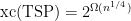
We solve a 20-year old problem posed by M. Yannakakis and prove that there exists no polynomial-size linear program (LP) whose associated polytope projects to the traveling salesman polytope, even if the LP is not required to be symmetric. Moreover, we prove that this holds also for the maximum cut problem and the stable set problem. These results follow from a new connection that we make between one-way quantum communication protocols and semidefinite programming reformulations of LPs.

The history of this problem is quite interested. From Gerd Woeginger’s P-versus-NP page (See also Mike Trick’s blog post on Swart’s attempts):

In 1986/87 Ted Swart (University of Guelph) wrote a number of papers (some of them had the title: “P=NP”) that gave linear programming formulations of polynomial size for the Hamiltonian cycle problem. Since linear programming is polynomially solvable and Hamiltonian cycle is NP-hard, Swart deduced that P=NP.

In 1988, Mihalis Yannakakis closed the discussion with his paper “Expressing combinatorial optimization problems by linear programs” (Proceedings of STOC 1988, pp. 223-228). Yannakakis proved that expressing the traveling salesman problem by a symmetric linear program (as in Swart’s approach) requires exponential size. The journal version of this paper has been published in Journal of Computer and System Sciences 43, 1991, pp. 441-466.

In his paper, Yannakakis posed the question whether one can show such a lower bound unconditionally, i.e., without the symmetry assumption and Yannakakis conjectured that symmetry ‘should not help much’. This sounded reasonable however no proof was known. In 2010, to the surprise of many, Kaibel, Pashkovich, and Theis proved that there exist polytopes whose symmetric extension complexity (the number of facets of the polytope) is super-polynomial, whereas there exists asymmetric extended formulations that use only polynomially many inequalities; i.e., symmetry does matter. On top of that, the considered polytopes were closely related to the matching polytope (used by Yannakakis to establish the TSP result) which rekindled the discussion on the (unconditional) extension complexity of the travelling salesman polytope and Kaibel asked whether 0/1-polytopes have extended formulations with a polynomial number of inequalities in general or if there exist 0/1-polytopes that need a super-polynomial number of facets in any extension. Beware! This is not in contradiction or related to the P-vs.-NP question as we only talk about the number of inequalities and not the encoding length of the coefficients. This was settled by Rothvoss in 2011 by a very nice counting argument: there are 0/1-polytopes that need a super-polynomial number of inequalities in any extension.

To make the following slightly more formal, let ${P \subseteq {\mathbb R}^n}$ be a polytope (of some dimension). Then an extended formulation for ${P}$ is another polytope ${Q \subseteq {\mathbb R}^\ell}$ such that there exists a linear projection ${\pi}$ with ${\pi(Q) = P}$ . The size of an extension ${Q}$ is now the number of facets of ${Q}$ and the extension complexity of ${P}$ (denoted by: ${\text{xc}(P)}$ ) is the minimum ${\ell}$ such that there exists an extension of size ${\ell}$ . We are interested in ${\text{xc}(P)}$ where ${P}$ is the travelling salesman polytope. Our proof heavily relies on a connection between the extension complexity of a polytope and communication complexity (the basic connection was made by Yannakakis and it was later extended by Faenza, Fiorini, Grappe, and Tiwary and Fiorini, Kaibel, Pashkovich, Theis in 2011). In fact, suppose that we have an inner and outer description of our polytope ${P}$ , say ${P = \text{conv}\{v_1, \dots v_n\} = \{x \in {\mathbb R}^n \mid Ax \leq b\}}$ . Then we can define the slack matrix ${S(P)}$ as ${S_{ij} = b_i -A_i v_j}$ , i.e., the slack of the vertices with respect to the inequalities. The extension complexity of a polytope is now equal to the nonnegative rank of ${S}$ which is essentially equivalent to determining the best protocol to compute the entries of ${S}$ in expectation (Alice gets a row index and Bob a column index). The latter can be bounded from below by the non-deterministic communication complexity and we use a certain matrix ${M_{ab} = (1-a^Tb)^2}$ which has large non-deterministic communication complexity (see de Wolf 2003). This matrix is special as it constitutes the slack for some valid inequalities for the correlation polytope which eventually leads to a exponential lower bound for the extension complexity of the correlation polytope. The latter is affine isomorphic to the cut polytope. Then via a reduction-like mechanism similar lower bounds are established for the stable set polytope ( ${\text{xc(stableSet)} = 2^{\Omega(n^{1/2})}}$ ) for a certain family of graphs and then we use the fact that the TSP polytope contains any stable set polytope as a face (Yannakakis) for suitably chosen parameters and we obtain ${\text{xc(TSP)} = 2^{\Omega(n^{1/4})}}$ .

Here are the slides:

Written by Sebastian

January 5, 2012 at 3:17 pm

Posted in Announcements, mathematics, Talks

Fundamental principles(?) in mathematics

with 2 comments

As said already in one of my previous posts, David Goldberg and I had a nice discussion about “fundamental concepts” in mathematics. Our definition of “fundamental” was that,

once seen you cannot imagine anymore having not known it beforehand and it completely changes your way of thinking and
a somewhat realistic approach, i.e., when subtracted from the “world of thinking” something is missing.

So here is our preliminary list of things that we came up with – in random order – and a very brief, (totally biased) meta-description of what we mean by these terms. Of course, this list is highly subjective! For each of these “fundamental concepts” the idea is to have (about) 3 applications and try to distill the main core. There will be (probably) a separate blog post for each point on the list.

Identity/Equality. Closely related to being isomorphic. The power of identity is so penetrating that I cannot even find a short explanation. Do I have to? (Aristotle’s first law of thought)
Contradiction. Showing that something cannot be true as it leads to a contradiction or inconsistency. Closely related to this is the principium tertii exclusi or law of the excluded third as this is how we often use proofs by contradiction: a statement holds under various assumptions because its negation leads to a contradiction. If you do not believe in the law of the excluded thirdthen you obtain a different logic/mathematics. In particular, in these logics, usually every proof also constitutes some form of an algorithm as existence by mere contradiction when assuming non-existence is not allowed. (see also Aristotle’s second/third law of thought)
Induction. Establishing a property by relying on the same property for smaller sub-objects.
Recursion. Somewhat dual to induction: a larger object is defined as a function of smaller objects that have been subject to the same construction themselves.
Fixpoint. The existence of a point that is invariant under a map. Equilibria in games.
Symmetry. The notion of symmetry. Take a cube – rotating it does not really change the cube.
Invariants. Think of the dimension of a vector space. Invariants are a powerful way to show that two things are not equal (or isomorphic).
Limits. What would we do without limits? The idea of hypothetically continuing a process infinitely long. Think of the definition of a derivative.
Diagonalization. One of my personal favorites. Constructing a member not being in a family by making sure it differs from all the members in the family at (at least) one position. Diagonalization often exploits self-references. An example is Cantor’s proof.
Double counting. You count a family of objects in two different ways. Then the resulting “amounts” have to be identical. Typical example is the handshaking in graphs.
Proof. The notion of proof is very fundamental. Once proven a statement remains true (provided constistency etc). Interestingly, it can be proven that some things cannot be proven. A good example for the latter is the existence of inaccesible cardinals which is consistent with ZFC.
Randomness. Randomness is an extremely fundamental concept. One of my favorite applications is probably the probabilistic method. Think about Johnson’s ${7/8}$ –approximation algorithm for 3SAT or the PCP theorem.
Algorithm. When considering a function ${f: M \rightarrow N}$ we are often not just interested in what ${f}$ computes but in particular howit can be computed. In this sense the algorithmic paradigm is an additional layer to the somewhat descriptive layer of classical mathematics.
Exponential growth. What we were particularly thinking about was the idea that a relative improvement bounded away from ${0}$ ensures exponentional progress. This is used regularly in different scaling algorithms such as barrier algorithms, potential reduction methods, and certain flow algorithms.
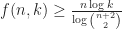
Information. The idea that often a critical amount of informationis necessary to decide a property. Then fooling set like arguments can show that the information is not sufficient. Prime examples include the classical example that sorting via comparison needs at least ${\Omega(n \log n)}$ comparisons, communication complexity, and query complexity.
Function/Relation. Mapping one set to another. In particular important when the function/relation is homogeneous, i.e., when it preserves the structure.
Density and approximation. The idea that a set (such as the reals) can be approximated arbitrarily well by an exponentially smaller set (such as the rationals). This exponential by polynomial approximation is also something that we are using in approximation algorithms, say, when we round the input. In this case the set of polytime solvable (rounded) instances is “dense” in the set of all instances. It can also be found in set theory when using prediction principles (such as Jensen’s diamond principle or Shelah’s Black Box) to predict functions on a stationary set by an exponentially smaller set.
Implicit definitions. The concept of defining something not in an explicit manner but as a solutionto a set of contraints.
Abstraction. The use of variables is so ingrained in us that we cannot even imagine to do serious mathematics without them. But abstraction is much more. It is the ability to see more clearly because we “abstract away” unnecessary details and we use “abstraction” to unify seemingly unrelated things.
Existence (in the sense that Brouwer hated). One of the keywords here is probably non-constructivism and the probabilistc methods and indirect arguments are two promiment methods in this category. This was something that Brouwer despised: the idea to infer, e.g., existence of something merely because the contrary statement would lead to a contradiction (Brouwer’s school of thought denies the tertium non datur). The probabilistic method might have been fine with him. Although that is not clear at all as on a deep level we are merely trading an existential quantifier for a random one… long story…
Duality. By duality we mean the wider idea of duality, i.e., for example the forall quantifier and the existential quantifier. Basically, when we talk about duality we often think about some structure describing the “space of positive statement” and a dual structure that describes the “space of negative statement”. In some sense duality is a form of a compact representation of the negation of a statement.
Counting. Counting is again something that penetrates every mathematical theory. My favorite application of counting is the Pigeonhole principle.
Hume’s principle (suggested by Hanno – see comments). Two quantities are the same if there exists a bijection between them. Somewhat related to “equality” however here we explicitly ask for the existence of a bijection. For example there are as many integers as their are rationals.
Infinity (suggested by Hanno – see comments). The idea that something is not finite. With the notion of infinity I feel that the notion of countably infinite and uncountably infinite is closely connected. In fact the Continuum Hypothesis (CH) is such a case. It is consistent with ZFC and asserts that the first uncountably infinite cardinal is the size of the power set of the natural numbers (essentially the reals), i.e., whether $\aleph_1 = 2^{\aleph_0}$ ). However in other models of set theory $\aleph_1 \neq 2^{\aleph_0}$ is possible, by adding, e.g., Cohen reals.

Written by Sebastian

January 2, 2012 at 8:49 pm

Posted in Crackpot halluzinations, mathematics, things that make me think

Tagged with contradiction, david goldberg, fundamental concepts, logics

Two good reads.

with one comment

Christmas time is reading time… and I actually read two quite amazing books:

Jacques Hadamard: The Psychology of Invention in the Mathematical Field
A classic. Very nice introspection and discussion about “how” mathematics is done. In particular it discusses a lot of potential theories of mathematical innovation and invention (as one might have guessed from the title).
Norbert Wiener: I Am a Mathematician
Part two of his autobiography. A very interesting read with a lot of big names and a lot of interesting insights into various aspects in and around mathematics. (thanks to Dave Goldberg for the pointer)

Written by Sebastian

December 29, 2011 at 10:44 pm

Posted in what else is out there

Tagged with Jacques Hadamard, Norbert Wiener, Psychology of Invention

Informs Annual Meeting 2011

leave a comment »

I plan to update this post in the course of the following days and I would have also loved to send out a few more tweets, especially now that I have this fancy twitter ribbon, but I have hard time connecting to the internet at the convention center.

Day 1: So the first day of the Informs Annual Meeting is almost over… What were my personal highlights from today? I listened to quite a lot of talks and most of them were really good so that I feel that it would not be fair to mention only a few selected ones. One personal highlight that I would like to mention though is the Student Paper Prize that Dan Dadush from Georgia Tech got for his work together with Santanu Dey and Juan Pablo Vielma on the Chvátal-Gomory closure for compact convex sets. This result is really amazing as it provides deep insights into the way of how cutting-plane procedures work when applied to non-linear relaxations. Congratulations Dan! Below is a picture of the three taken at the session.

Day 2: The second day of the Informs meeting was great. In particular I loved the integer optimization session (for apparent reasons) and had some extremely intense and deep discussions with some of my colleagues – for me this is the most important reason to go to a conference: dialog. One such discussion was with David Goldberg from GATech about the fundamental concepts in optimization/math/reasoning that completely redefine your thinking once fully understood/appreciated (this includes concepts such as “equality”, “proof by contradiction”, “induction”, or “diagonalization”). I will have a separate blog post together with David on that. If you think there is a concept that completely changed your thinking, please email us or drop us a line in the comment section. I am off to my talk now – more later…

Day 3: I actually did not see too much of the third day as I had to leave early.

All in all, Informs 2011 was a great event, in particular to meet all the people that are usually spread all over the US. I was actually quite happy to see that there were also quite a lot of Europeans at the conference

Written by Sebastian

November 13, 2011 at 9:09 pm

Posted in Mathematics and Optimization

Tagged with annual meeting, Informs, optimization

UniGestalten initiative (Germany-specific)

leave a comment »

The ‘Die Junge Akademie’ together with the ‘Stifterverband der Deutschen Wissenschaft’ has launched the very interesting initiative ‘UniGestalten’ to improve working and living at German universities. People can submit and discuss ideas for improving various aspects of teaching, research, administration, and more. From the homepage of the initiative (German):

Wir brauchen Leute, die vor- und nachdenken.
Für neue Perspektiven zum Leben und Arbeiten an der Uni!

Unser Ziel ist es, neue Perspektiven für den Alltag an unseren Hochschulen auszuloten und konkrete Lösungsvorschläge zu entwickeln. Wir wollen zeigen, dass nicht nur große strukturelle Entscheidungen in Wissenschaft, Wirtschaft und Politik etwas verändern können, sondern dass jeder Einzelne etwas bewegen kann. Wir setzen auf die Innovationskraft von Personen und auf die Lernfähigkeit der Organisation. Wir erwarten keinen allumfassenden Masterplan. Im Gegenteil: Wir glauben daran, dass auch kleine Ansätze viel verändern können. Von den Studierenden und Ehemaligen, über Lehrende und Forschende, Beschäftigte aus Technik und Verwaltung, bis hin zu den Partnern aus der Wirtschaft – jeder Einzelne hat seine eigenen Erfahrungen im Unibetrieb gesammelt und kann mit konkreten Ideen das Leben und Arbeiten an der Hochschule von morgen gestalten.

Ihr Beitrag kann eine ganz persönliche Initiative sein, ein konkreter Verbesserungsvorschlag oder ein interessantes Geschäftsmodell. Ihre Kommentare zu den Beiträgen sind uns jedoch genauso wichtig,

um die eingereichten Ideen weiterzuentwickeln. Jeder ist ein Teil dieser CommUNIty!

So if you happen to life/work/study at a German university you should definitely have a look and maybe even submit your own idea.

Written by Sebastian

November 6, 2011 at 10:14 am

Posted in Announcements

Tagged with "Die Junge Akademie", "Stifterverband der Deutschen Wissenschaft", Education, German, Germany, Hochschule, Leben, unigestalten

indirect proofs: contrapositives vs. proofs by contradiction

leave a comment »

Last week I read a rather interesting discussion on contrapositives vs. proofs by contradiction as part of Timothy Gowers’ Cambridge Math Tripos, mathoverflow, and Terry Tao’s blog. At first sight these two concepts, the contrapositive and the reductio ad absurdum (proof by contradiction) might appear to be very similar. Suppose we want to prove $A \Rightarrow B$ for some statements $A$ and $B$ . Then this is equivalent to showing $\neg B \Rightarrow \neg A$ (at least in classical logic). The latter is the contrapositive and often it is easier to go with the contrapositive. In the case of the indirect proof we do something similar, however there is a slight difference: we assume that $A \wedge \neg B$ and deduce a contradiction. So what the big deal? The difference seems to be more of a formal character. However this is not true. In the first case we remain in the space of “true statements”, i.e., any deduction from $\neg B$ is a consequence of $A$ that we can use later “outside of the proof”. In the case of the proof by contradiction we move in a “contradictory space” (as $A \wedge \neg B$ is contradictory) and everything that we derive in this space is potentially garbage. Its sole purpose is to derive a contradiction however as we work in a contradictory system we cannot guarantee that the statement derived within the proof are true statement; in fact they are likely not be true as they should result in a final contradiction.

Interestingly a similar phenomenon is known for cutting-plane procedures or cutting-plane proof systems (both terms essentially mean the same thing; it is just a different perspective) . Let me give you an ultra-brief introduction of cutting-plane procedures. Given a polytope $P \subseteq [0,1]^n$ we are often interested in the integral hull of that polytope which is defined to be $P_I = \text{conv}(P \cap \{0,1\}^n)$ . A cutting-plane procedure $M$ is now a map that assigns to $P$ a new polytope $M(P)$ such that $P_I \subseteq M(P) \subseteq P$ and $M(P)$ hopefully provides a tighter approximation of $P_I$ . So what the cutting-plane procedure does, is to derive new valid inequalities for $P_I$ by examining $P$ and usually the derivation is computationally bounded (otherwise we could just guess the integral hull); the exact technical details are not too important at this point.

Now any well-defined cutting-plane procedure $M$ satisfies $M(P \cap \{cx \le \delta\}) \subseteq M(P) \cap \{cx \le \delta\}$ . Or put differently, giving the cutting-plane procedure access to an additional inequality can potentially increase the strength of the procedure as compared to let it work on $P$ and then intersect with the half-space $cx \leq \delta$ afterwards. Now what does this have to do with indirect proofs and contrapositives? The connection arises from the following trivial insight: an inequality $cx \leq \delta$ (with integral coefficients and right-hand side) is valid for $P_I$ if and only if $(P \cap \{cx \geq \delta + 1 \})_I = \emptyset$ . In particular a sufficient condition for the validity of $cx \leq \delta$ for $P_I$ is $M(P \cap \{cx \geq \delta + 1 \}) = \emptyset$ . The key point is that $M(P \cap \{cx \geq \delta + 1 \})$ can be strictly contained in $M(P) \cap \{cx \geq \delta + 1 \}$ . The first one is the indirect proof, whereas the second one is the contrapositive, as we verify the validity of $cx \leq \delta$ by testing if $M(P) \cap \{cx \geq \delta + 1 \} = \emptyset$ . However we do not use the inequality $cx \leq \delta$ in the cutting-plane procedure, i.e., the procedure has no a priori knowledge about what to prove, whereas in the case of indirect proofs, we add the negation of $cx \leq \delta$ and the procedure can use this information.

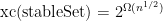
So how much do can you gain? Suppose we have a graph $G= (V,E)$ and we consider the associated fractional stable set polytope $FSTAB(G) = \{ x \in [0,1]^V \mid x_u + x_v \leq 1 \ \forall\; (u,v) \in E\}$ . Typically (there are a few exceptions), for a classical cutting-plane procedure the derivation of clique inequalities is involved and we need $\Omega(\log k)$ applications of the cutting-plane procedure to derive the clique inequalities for a clique $C$ of size $k$ , i.e., $\sum_{v \in C} x_v \leq 1$ . However an indirect proof of the clique inequalities takes only a single application of the most basic cutting-plane operator: Consider

$FSTAB(G) \cap \{\sum_{v \in C} x_v \geq 2\} =: Q$

for a clique $C$ . It is not hard to see that $Q \cap \{x_v = 1\} = \emptyset$ for all $v \in C$ . A basic derivation that any sensible cutting-plane operator $M$ supports is to derive that $x_i \leq 0$ , i.e., $x_i \leq 0$ is valid for $M(Q)$ whenever $x_i < 1$ is valid for $P$ . Therefore we obtain that $M(Q) \subseteq \bigcap_{v \in C} \{ x_v = 0\}$ . On the other hand $M(Q) \subseteq \{\sum_{v \in C} x_v \geq 2\}$ and so $M(Q) = \emptyset$ holds and thus the indirect proof derived $\sum_{v \in C} x_v \leq 1$ .

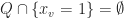
So what one can see from this example is that indirect proofs (at least in the context of cutting-plane proof systems) can derive strong valid inequalities in rather few rounds and outperform their direct counterpart drastically (constant number of rounds vs. log(n) rounds). However a priori knowledge of what we want to prove is needed in order to apply the indirect proof paradigm. This makes it hard to exploit the power of indirect proofs in cutting-plane algorithms. After all, you need to know the “derivation” before you did the actual “derivation”. Nonetheless, in some cases we can use indirect proofs by guessing good candidates for strong valid inequalities and then verify their validity using an indirect proof.

Check out the links for further reading:

Written by Sebastian

October 18, 2011 at 8:01 pm

Posted in Mathematics and Optimization, things that make me think

Tagged with contrapositives, cutting-plane procedures, indirect proofs, proof systems

Mastermind – five questions do suffice

leave a comment »

Today I would like to talk about the Mastermind game and related (recreational?!) math problems – the references that I provide in the following are probably not complete. Most of you might know this game from the 70s and 80s. The first player is making up a secret sequence of colored pebbles (of a total of 6 colors) and the other player has to figure out the sequence by asking questions about the code by proposing potential solutions. The first player then indicates the number of color matches.

Mastermind (source: Wikipedia)

More precisely, Wikipedia says:

The codebreaker tries to guess the pattern, in both order and color, within twelve (or ten, or eight) turns. Each guess is made by placing a row of code pegs on the decoding board. Once placed, the codemaker provides feedback by placing from zero to four key pegs in the small holes of the row with the guess. A colored (often black) key peg is placed for each code peg from the guess which is correct in both color and position. A white peg indicates the existence of a correct color peg placed in the wrong position.

If there are duplicate colours in the guess, they cannot all be awarded a key peg unless they correspond to the same number of duplicate colours in the hidden code. For example, if the hidden code is white-white-black-black and the player guesses white-white-white-black, the codemaker will award two colored pegs for the two correct whites, nothing for the third white as there is not a third white in the code, and a colored peg for the black. No indication is given of the fact that the code also includes a second black.

Once feedback is provided, another guess is made; guesses and feedback continue to alternate until either the codebreaker guesses correctly, or twelve (or ten, or eight) incorrect guesses are made.

In a slightly more formal way, we have a string in $\{1,...,6\}^4$ and the “decoder” wants to reconstruct this string by inferring from the provided feedback. One of the natural questions that arise is of course how many questions do suffice. Knuth [Knuth76] then showed that five questions suffice to be able to always reconstruct the secret string. What is interesting about the proof is that it is a “table” – basically output of a computer program. This lookup table can be used so find a next question at any given point. The table is a greedy optimization in some sense: “Figure 1 [the lookup table] was found by choosing at every stage a test pattern that minimizes the maximum number of remaining possibilities, over all 15 responses by the codemaker”.

Later in 1983, Vasicek Chvátal dedicated a paper on the Mastermind game to Paul Erdős for his 70th birthday. Chvátal looked at generalized admissible Mastermind vectors denoted by $V(n,k)$ of vectors of length n with k different colors. It is not too hard to see that the minimum number of questions $f(n,k)$ needed to correctly identify any string in $V(n,k)$ is bounded from below by

$f(n,k) \geq \frac{n \log k}{\log \binom{n+2}{2}}$

which arises from the fact that there are only $\binom{n+2}{2}$ different answers and $n^k$ different strings have to be distinguished. Complementing this bound, Chvátal showed that the number of questions needed to be asked without waiting for the answer (i.e., the questions are asked in one go, then the answers to all questions are provided at once, and then the code has to be uniquely identified) can be bounded from above as follows: the number of questions needed for this static case will be denoted by $g(n,k)$ and for any $\epsilon > 0$ there exists $n(\epsilon)$ so that for all $n > n(\epsilon)$ and $k < n^{1-\epsilon}$ we have

$g(n,k) \leq (2+ \epsilon) n \frac{1+2 \log k}{\log n - \log k}$

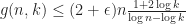
and clearly we have $f(n,k) \leq g(n,k)$ . The proof uses the probabilistic method in a nice way. Moreover, Chvátal also provides some upper and lower bounds for special cases. Those of you guys that know about my addiction to the Chvátal-Gomory closure and its friends might have already guessed that this is exactly how I came across the problem…

The latter problem where we do not wait for the answers is usually called the static mastermind problem whereas the classical version is called the dynamic mastermind problem. Later in 2003 and 2004 Goddard (see [Godd03,04]) provided optimal values for the minimal number of questions to be asked both in the dynamic as well as static case and also for the average number (denoted by $r(n,k)$ ) of questions needed whenever the secret string is uniformly picked at random. With the notation from above we have the following number of questions (tables taken from [Godd03,04]):

For the average number of queries needed ( $r(n,k)$ ) we obtain:

		Positions
		2	3	4	5	6	7
Colors	2 –	2	2.250	2.750	3.031	3.500	3.875
	3 –	2.333	2.704	3.037	3.358
	4 –	2.813	3.219	3.535
	5 –	3.240	3.608	3.941
	6 –	3.667	3.954	4.340
	7 –	4.041	4.297
	8 –	4.438
	9 –	4.790
	10-	5.170

and similarly for the dynamic case we have the following minimum number of queries $f(n,k)$ :

		Positions
		2	3	4	5	6	7	8
Colors	2 –	3	3	4	4	5	5	6
	3 –	4	4	4	4	5	<= 6
	4 –	4	4	4	5	<= 6
	5 –	5	5	5	<= 6
	6 –	5	5	5
	7 –	6	6	<= 6
	8 –	6
	9 –	7
	10-	7

and for the static case $g(n,k)$ we have the following table. Note that in the table below the final “query” that states the recovered string is not counted as in comparison to the ones above. Therefore in order to compare the values with the ones above you need to add “1” to each entry.

		Positions
		2	3	4	5	6	7	8
Colors	2 –	2	2	3	3	4	5	5
	3 –	2	3	3	4	4	<= 5
	4 –	3	4	4	5
	5 –	4	4	5
	6 –	4	5	6
	7 –	5	6	<= 7
	8 –	6	7	<= 8
	9 –	6	8
	10–	7	9

(there seems to be a typo for n = 2 and k = 3 in one of the tables, as the static case has a better performance than the dynamic case which is not possible).

In order to be able to actually check (with a computer) whether a certain number of questions suffices, we have to exclude symmetries in a smart way. Otherwise the space of potential candidates is too large. In this context, in particular the orderly generation framework of [McKay98] is very powerful. The idea behind that framework is to incrementally extend the considered structures in such a way that we only add a canonical candidate per orbit. Moreover, after having extended our structure to the next “size” we need to check whether it is isomorphic to one of the previously explored structures. In this case we do not consider it. For each candidate we check whether the number of distinct answers is equal to the total number of possible secret codes. In this case there is a bijection between the two and therefore we can decode the code. However it is not clear that this bijection needs to have a “nice” structure or that it is “compact” in some sense.

References:

[Knuth76]: Knuth, D.E. 1976. “The computer as a master mind.” Journal of Recreational Mathematics. http://colorcode.laebisch.com/links/Donald.E.Knuth.pdf (Accessed June 9, 2011).
[Chvátal83]: Chvátal, V. 1983. “Mastermind.” Combinatorica 3: 325-329.
[McKay98]: McKay, B.D. 1998. “Isomorph-free exhaustive generation.” Journal of Algorithms 26(2): 306–324.
[Good03]: Goddard, W. 2003. “Static Mastermind.” Journal of Combinatorial Mathematics and Combinatorial Computing 47: 225-236
[Godd04]: Goddard, W. 2004. “Mastermind Revisited.” Journal of Combinatorial Mathematics and Combinatorial Computing 51: 215-220

Written by Sebastian

October 13, 2011 at 4:20 pm

Posted in what else is out there

Tagged with Donald Knuth, Journal of Recreational Mathematics, Mastermind, Paul Erdős

Steve Jobs 1955-2011

leave a comment »

Thank you for providing us not just with different tools but with a different way to think.

You inspired all of us.

We will miss you very much!

Written by Sebastian

October 6, 2011 at 8:41 am

Posted in things that make me think

Tagged with Apple, steve jobs

Sebastian Pokutta's Blog

On the polyhedral inapproximability of the SDP cone

The Scottish Café revisited

On linear programming formulations for the TSP polytope

Fundamental principles(?) in mathematics

Two good reads.

Informs Annual Meeting 2011

UniGestalten initiative (Germany-specific)

indirect proofs: contrapositives vs. proofs by contradiction

Mastermind – five questions do suffice

Steve Jobs 1955-2011

Recent Posts

Shared items

Categories

Archives

Pages

Top Posts

Meta

Email Subscription