Information asymmetry and beating the market

Recently, I was wondering how much money you can effectively gain by investing, given a certain information advantage: Suppose that you want to invest some money, for the sake of simplicity say $10,000. Can you assume to be able to extract an average-exceeding return from the market given that you have an information advantage? If you believe in the strong form of the efficient market hypothesis then the answer is no of course. If not, then is it at least theoretically possible?

Let us consider a simplified setting. Suppose that we can invest (long/short) in a digital security (e.g., digital options) with payouts 0 and 1 (with a price of 0.5) and let us further suppose that it pays out 1 with a probability of 50%. Now assume that we have a certain edge over the market, i.e., we can predict the outcome slightly more accurately, say with accuracy. If we have a good estimate of our edge, we can use the Kelly Criterion to allocate our money. The Kelly Criterion, named after John L. Kelly, Jr determines the proportional amount of money to bet from own bankroll so that the overall utility is maximized – this criterion is provably optimal. It was presented by Kelly in his seminal 1956 paper “A New Interpretation of Information Rate“. In this paper Kelly links the channel capacity of a private wire (inside information) to the maximum amount of return that one can extract from a bet. While this bound is a theoretical upper bound, it is rather strong in its negative interpretation: If you do not have any inside information (which includes being just smarter than everybody else or other intangible edges) you cannot extract any cash. The Kelly Criterion arises as an optimal money management strategy derived from the link to Shannon‘s Information Theory and in its simplest form it can be stated as:

where are the odds, the probability to win, and the probability to lose. So in our setting, where we basically consider fair coin tosses whose outcomes we can predict with accuracy, an edge of 1% or 100bps is considerable. Using the money management strategy from above (neglecting taxes, transaction fees, etc.), we obtain:

100bp edge

with an initial bankroll of $10,000, y-axis is log10(bankroll), x-axis is #bets. The five lines belong to the %5, 25%, 50%, 75%, and 95% percentiles computed on the basis of 5,000 Monte-Carlo runs. So even the 5% percentile sees a ten-fold increase of the bankroll after roughly 4,100 bets, whereas the 95% percentile is already at a 100-fold increase. In terms of real deals the number of bets is already considerable though — after all, which private investor does 4,000 transactions??

Unfortunately, an edge of 100bp is very optimistic and for, say, for 50bp edge the situation already looks a quite different: the 50% percentile barely reaches a ten-fold increase after 10,000 bets.

50bp edge

And now let us come to the more realistic scenario when considering financial markets. Here an edge of 10bp is already considered significant. Given all the limitations as a private investor, i.e., being further down the information chain, sub-optimal market access, etc., assuming an edge of 10bp would be still rather optimistic. In this case, using an optimal allocation of funds, we have the following:

10bp edge

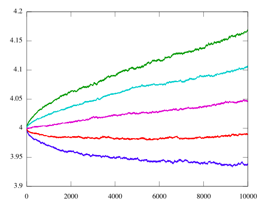
Here the 25% percentile actually lost money and even the 50% percentile barely gained anything over 10,000 bets. In the long run also here a strictly positive growth occurs, but for 10bp it takes extremely long: While you might be able do 4,000 deals over the course of say 10 – 30 years. Here even after 100,000 bets the 5% percentile barely reaches a 29% gain (over 100,000 bets!!). Given transaction costs, taxes, fees, etc., in reality the situation looks worse (especially when considered more complicated financial structures). So it comes all down to the question, how large your edge is.

Although extremely simplified here, a similar behavior can be shown for more complicated structures (using e.g., random walks).